introduction

In this post I’m going to explore using Python and Numpy to manipulate a jpg image, and do some of the kinds of transformations that you might normally do in a graphics design tool like Photoshop or Paint!

Why? Because we can! And by doing this, we will understand a lot more about computer based images, which will give us the basic foundation to understand what DALL-E and similar AI tools are doing with their magic and fairy dust - when we get to that stage.

I’ll be using some python packages I haven’t played with before. Skimage to import the image file, and matplotlib to render it so I can see what’s happening as the code progresses. I’ll be using the typical naming conventions for these packages, to make it easier for people familiar with them to read the code.

the jpg image format

First, a bit of background and context. JPG or JPEG stands for Joint Photographic Experts Group, which is the name of the committee that created the JPEG standard file format. JPG is one of the most common image file formats used for digital photos and images on the web.

At a basic level, JPG images work by compressing photographic image data to reduce the file size. This allows the images to take up less storage space and transmit faster across the internet.

The compression happens in a few key steps:

• The image is divided into blocks of 8x8 pixels.
• Each block goes through a mathematical transformation called the Discrete Cosine Transform (DCT). This converts the pixel values into frequency components.
• The higher frequency components, which are less visible to the human eye, are discarded. This is where the lossy compression happens.
• The remaining components are quantised - converted into integer values that can be efficiently encoded.
• The quantised values are encoded and compressed using a technique called run-length encoding. This further reduces redundant data.
• The compressed data is stored in the JPG file along with some header information like image size.
• When the JPG is opened again, the process is reversed - the image data is extracted, decoded, de-quantised and reconstructed into an approximation of the original image.

The amount of compression (and loss of quality) can be adjusted when saving the JPG. Higher quality JPGs compress less by retaining more high frequency components. Lower quality JPGs compress more and lose finer details and resolution.

So in summary, JPG compression works by selectively discarding fine details that are less visible to the human eye, allowing the images to take up less digital storage and transmission space.

jpg images in numpy

When jpg images are opened using Numpy, they are converted to a 3D Numpy array.

Think of a Rubik’s Cube, where one dimension of the cube represents the width of an image (in this case 3), with indexes 0, 1 and 2, one dimension represents the height of an image (also 3), and the third dimension (front to back, say) represents the colour intensity on 3 channels, Red, Green and Blue. Reminder: Numpy arrays are indexed from zero.

So this Rubik’s cube could represent a 3 x 3 pixel image, containing 9 pixels.

• The front panel of cubes could represent the red intensity of each of the 9 pixels, at position 0 in the array on the front to back dimension.
• The back panel of cubes could represent the blue intensity of each of the pixels, at position 2 in the array.
• The middle section of cubes sandwiched between the front and back, would represent the green intensity of each of the 9 pixels, at position 1 in the array on the front to back dimension.

All the colours of the image are then made up of the combination of the 3 colour intensities, front to back, for each pixel.

today’s challenge - manipulating a jpg image.

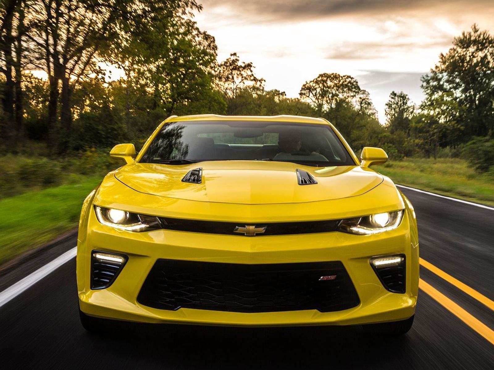
Let’s start with our basic image file which is a jpeg file of photograph of a yellow Camaro car, speeding along on the wrong side of the road.

We’re going to use the Numpy package for most of our work here, but we need a couple of other packages as well. We’re going to use the skimage package to read in our image, and we’re also going to use a package called matplotlib to display our image as we manipulate it. So, we need to import those.

First thing we need to do is import the jpg image. For this we will use the skimage io function imread. Then we’ll have a look at what we have within Python.

import numpy as np
from skimage import io
import matplotlib.pyplot as plt

camaro = io.imread("camaro.jpg")
print(camaro)

>>> [[[ 83  81  43]
>>>   [ 57  54  19]
>>>   [ 34  31   0]
>>>   ...
>>>   [179 144 112]
>>>   [179 144 114]
>>>   [179 144 114]]

>>>  [[ 95  93  55]
>>>   [ 72  69  34]
>>>   [ 46  43   8]
>>>   ...
>>>   [181 146 114]
>>>   [181 146 116]
>>>   [182 147 117]]

>>>  [[101  99  61]
>>>   [ 88  85  50]
>>>   [ 67  63  28]
>>>   ...
>>>   [184 149 117]
>>>   [184 149 117]
>>>   [184 149 119]]

As we can see, it has imported the jpg image as just a 3D Numpy array! But that makes sense if you think about it, as images are basically just numbers representing the intensity of each pixel, and in a colour image we have intensity values for each of the colour channels: red, green and blue.

Now, if we look at the shape of our image array, we can see the structure of our image.

print(camaro.shape)

>>> (1200, 1600, 3)

We see that it has a shape of 1200 x 1600 x 3.

This is telling us that the image, in the form of a 3D array,

• has 1200 rows of pixels,
• 1600 columns of pixels,
• and 3 colour channels, representing red, green and blue intensities of each pixel.

So, the image is wider than it is high, and each pixel is represented by its position on the picture (row & column number) and a number representing the intensity of each of the colours: red, green and blue.

So now we understand this data structure, we can use simple maths on the array to play around with the image, and Numpy makes this very easy.

cropping images

Say, we want to crop the image so we just have the car without all the background? We just have to slice the row and column parts of the array to show just the range of rows and columns we want to keep.

We will need only the pixels from rows 350 to 1100. We will need only the pixels from columns 200 to 1400.

I’ll also save the file so I can show you.

cropped = camaro[350:1100, 200:1400, :]
plt.imshow(cropped)
plt.show()
io.imsave("camaro_cropped.jpg", cropped)

So, here, we’re taking rows 350 - 1100, and columns 200 - 1400, and everything from the colour channels, out of our original image and creating a new image with just that section.

Here’s the cropped image:

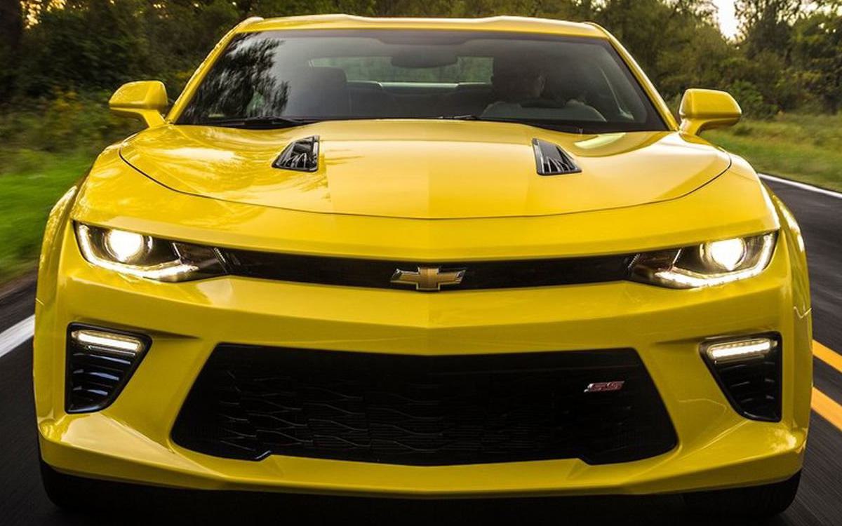
There we are, image cropped!

flipping images

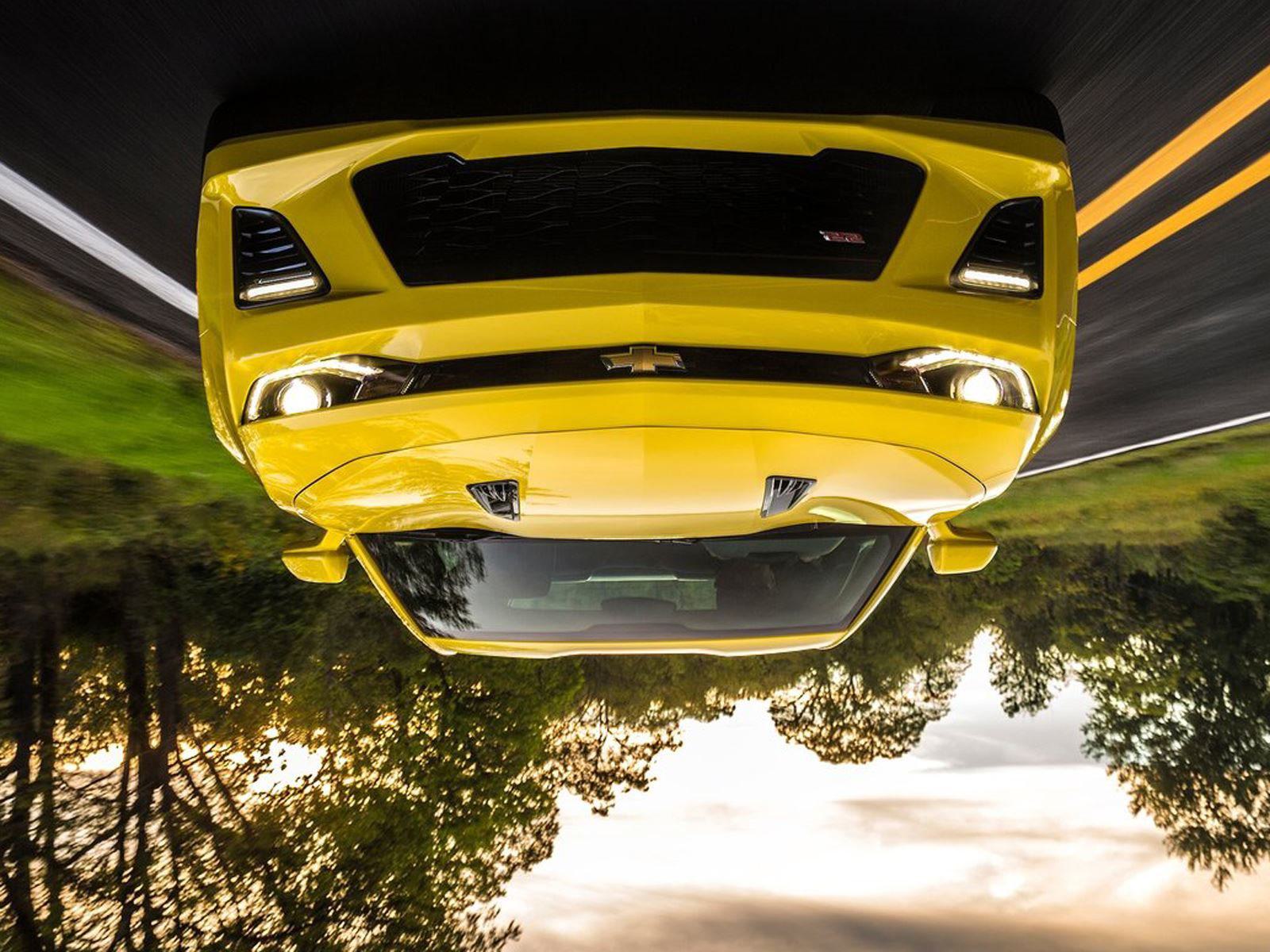
If we want to flip an image on the vertical axis, so it is upside down, what do you think we need to do? That’s right, we maths it! Numpy makes this really easy too, as you can see.

vertical_flipped = camaro[::-1, :, :]
plt.imshow(vertical_flipped)
plt.show()

io.imsave("camaro_vertical_flipped.jpg", vertical_flipped)

So, what’s this array code doing?

Basically the ::-1 part says take every row but in reverse! The other two parts say: take every column, and take every colour channel.

So we end up with our car flipped on its roof! Which is likely to happen if it keeps driving on the wrong side of the road.

mirror images

What we can flip vertically, we can of course flip horizontally as well. We just need to reverse the order of the columns instead of the rows.

horizontal_flipped = camaro[:, ::-1, :]
plt.imshow(horizontal_flipped)
plt.show()

io.imsave("camaro_horizontal_flipped.jpg", horizontal_flipped)

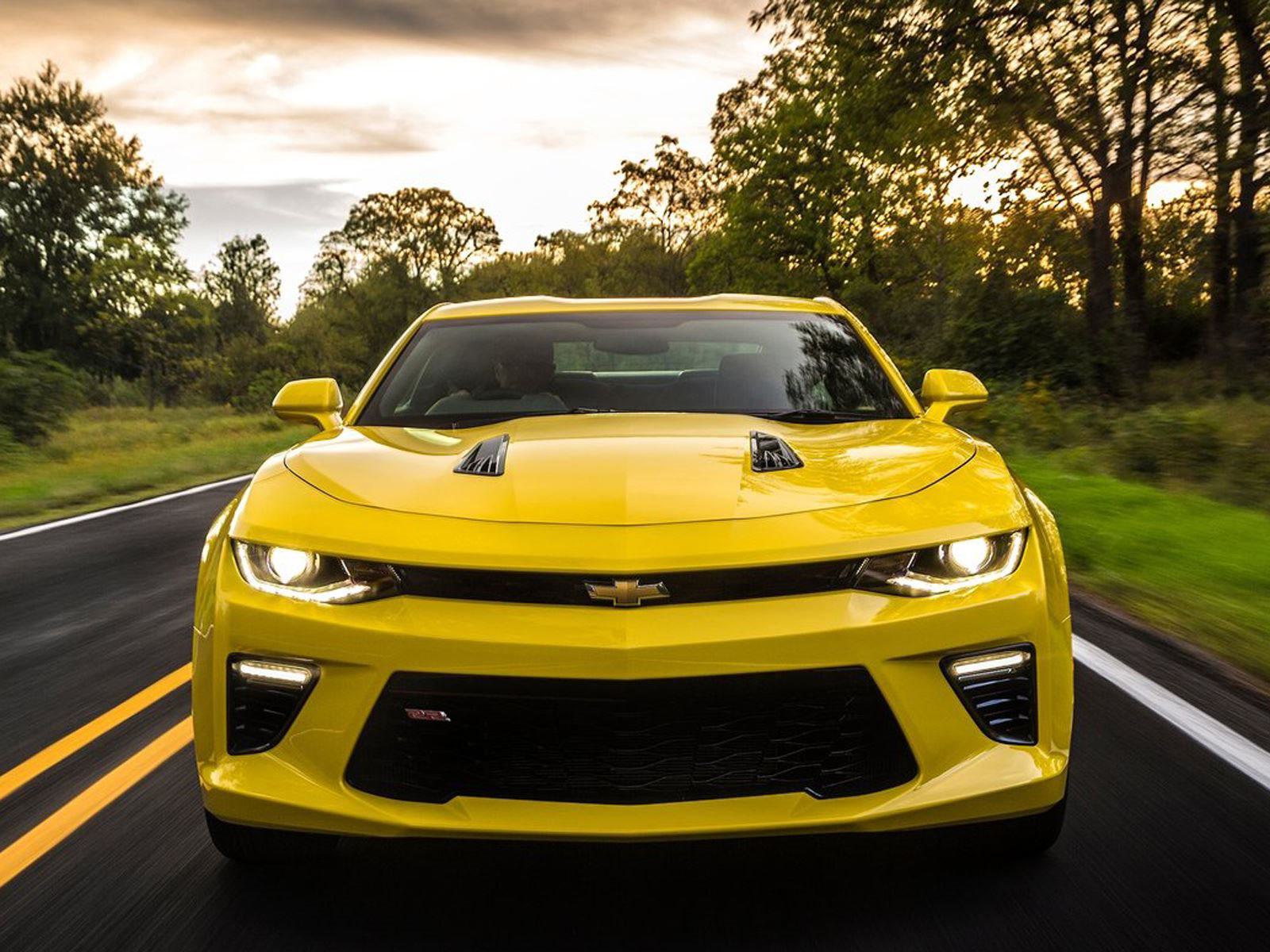
Now the car is driving on the correct side of the road! I feel safer already. Although, where is the camera-man standing? I’m not sure he survived!

colour channels

Right, it’s time to get a bit arty and start messing with the colour channels.

I’m going to split out the colour channels to create 3 images of my car, and then glue them together in a rainbow array. I’ll save all the images to files so you can see them on the blog. I can see them in the spydery-thing anyway using matplotlib, but sharing is caring, and this is starting to look amazing, so I wouldn’t want you to miss it!

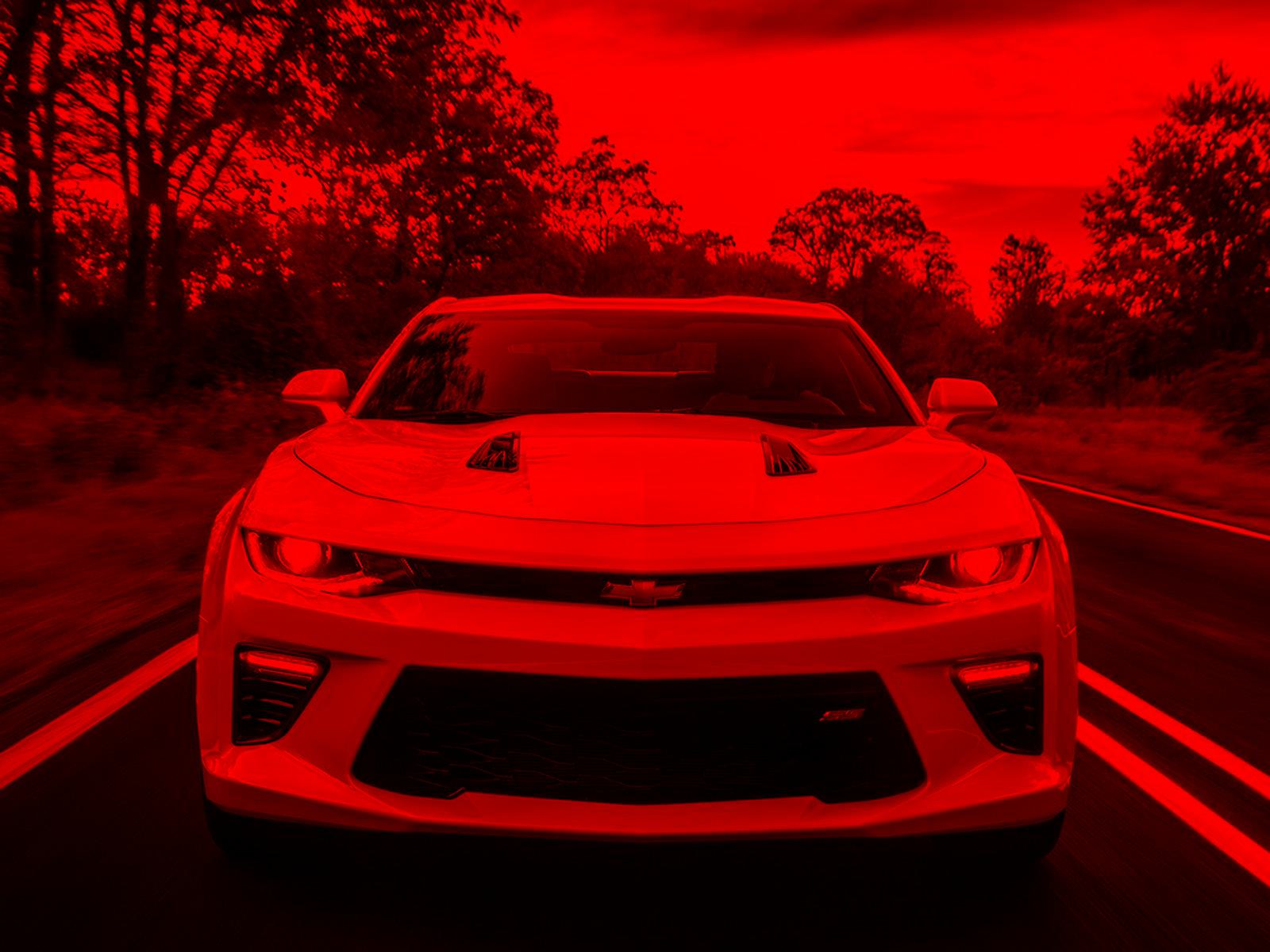
# select the red only channels from the camaro image array

# create a new array of the same 3D shape and unsigned integer data-type, and fill it with zeros
red = np.zeros(camaro.shape, dtype="uint8")

# copy over the Red intensity values only, from the original image.  Red is item [0] in the 3rd dimension.
red[:, :, 0] = camaro[:, :, 0]
plt.imshow(red)
plt.show()
io.imsave("camaro_red.jpg", red)

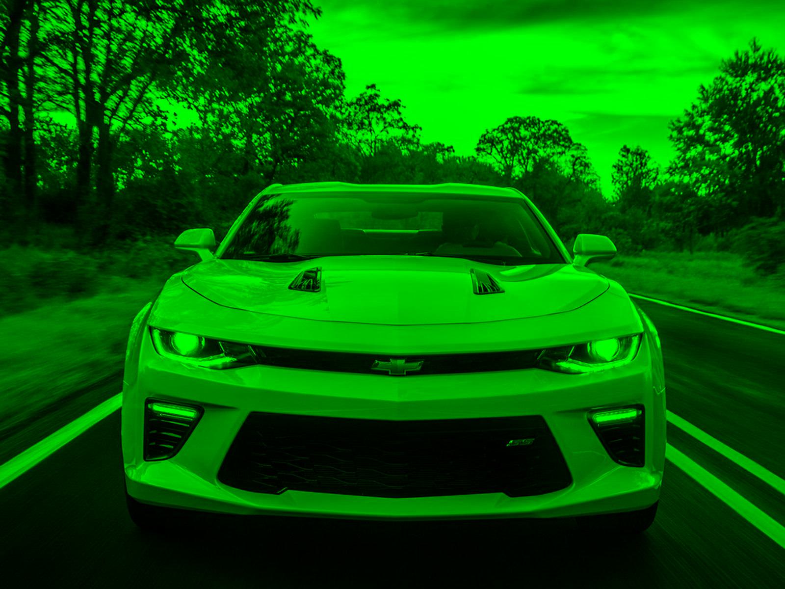
# select the green only channels from the camaro image array

# create a new array of the same 3D shape, and fill it with zeros
green = np.zeros(camaro.shape, dtype="uint8")

# copy over the Green intensity values only, from the original image.  Green is item [1] in the 3rd dimension.
green[:, :, 1] = camaro[:, :, 1]
plt.imshow(green)
plt.show()
io.imsave("camaro_green.jpg", green)

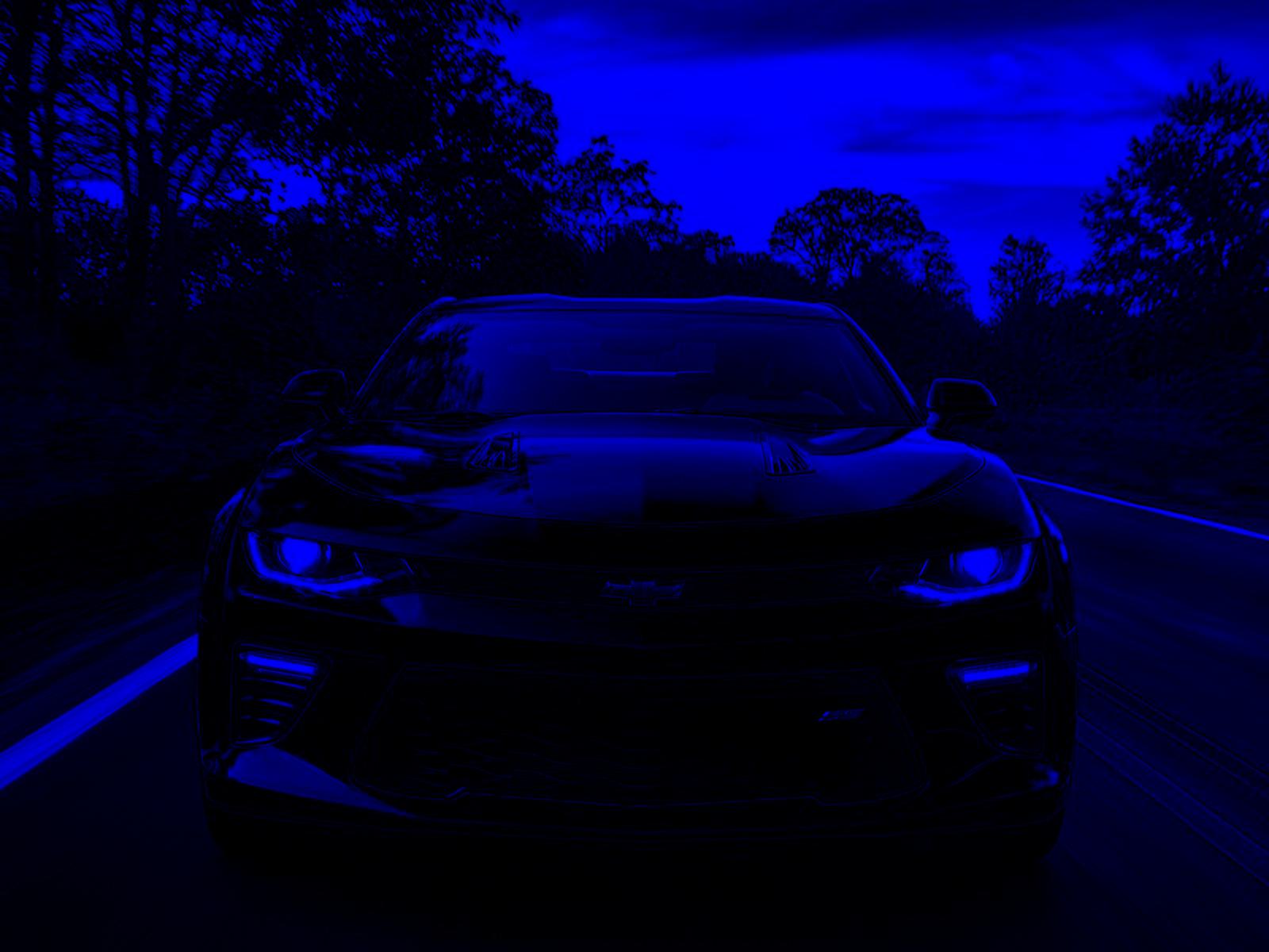
# select the blue only channels from the camaro image array

# create a new array of the same 3D shape and fill it with zeros
blue = np.zeros(camaro.shape, dtype="uint8")

# copy over the blue intensity values only, from the original image.  Blue is item [2] in the 3rd dimension.
blue[:, :, 2] = camaro[:, :, 2]
plt.imshow(blue)
plt.show()
io.imsave("camaro_blue.jpg", blue)

make a stack!

Now, we just stack our 3 different coloured arrays, one on top of the other to make a single stacked image array, that an arty person might print out and hang on their wall! We’ll use the vertical stack function, vstack for that.

camaro_rainbow = np.vstack((red, green, blue))
plt.imshow(camaro_rainbow)
plt.show()
io.imsave("camaro_rainbow.jpg", camaro_rainbow)

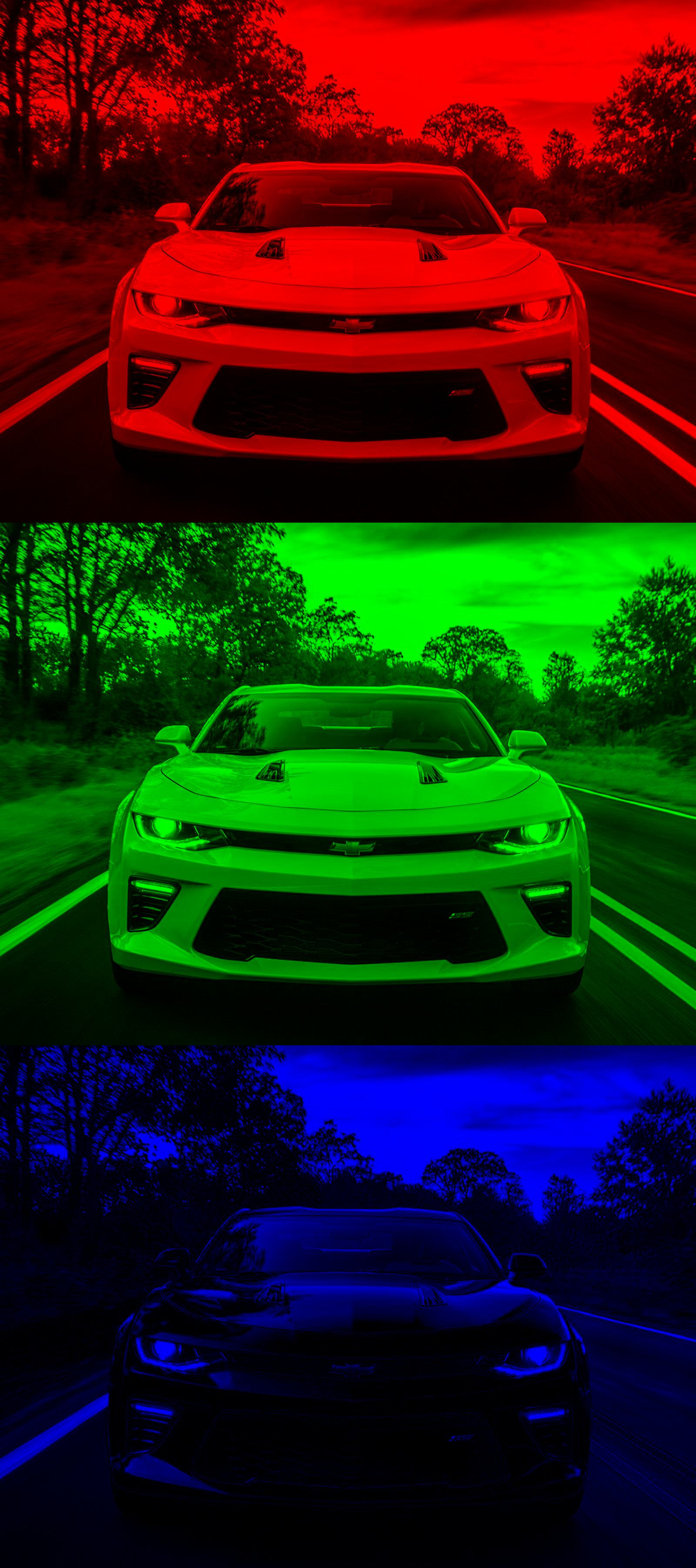
Move over Andy Warhol, this art stuff is really just maths!

random dad joke alert

# Q. Why don't JPG files make good accountants?

# A. Because they tend to lose a lot of details in the compression process.

I hope you have enjoyed this investigation of jpg image manipulation using Numpy arrays and Python. Numpy is really making some of this stuff look like childs-play! I hope to see you on our next intrepid Python adventure.